I recently completed a course on Supervised Machine Learning: Regression and Classification on Coursera, and in this post, I will try and summarize some of the concepts and interesting ideas. And no, this introduction was not written by chat GPT!
Machine Learning has taken off in the past decade due to an increase in available data and the computing power required to make meaningful predictions from it. The core function of Machine Learning and all its tools is ultimately to make good predictions and there are 2 distinct models that achieve this: Supervised and unsupervised (although there are many other machine learning algorithms these 2 build the foundation of machine learning).
In unsupervised learning the training data does not have labelled input and output pairs. The data that trains the model is uncategorized and the model is responsible for finding patterns in the data to make accurate predictions. Your Netflix and Amazon recommenders are good examples of unsupervised learning models.
As the name suggests, in supervised learning the training data has input and output pairs (X, Y). The model gets trained on the data that is correct and it is then used to make predictions with new data. If you have labelled data, supervised learning algorithms are usually the simplest to make predictions.
Supervised learning algorithms fall into 2 categories: regression and classification.
Regression
In a regression algorithm the model fits a curve to the data using linear regression which can then be used to predict the output based on new and unlabeled input. Regression predicts output values and I like to think of it as an ‘analog’ predictor, which essentially means that it can output a range of numbers. E.g., A model that predicts house prices based on input features such as location, age. etc.
The simplest function of linear regression is: f(X) = W*X + B, where W and B are the parameters and X is the feature. NOTE: The function is linear with respect to the parameters (w,b) and x can be of higher order. A simple way to think about features is that they are based on the training data’s inputs (e.g., size, price, weight etc.) and the parameters are what the algorithm optimizes to result in the best fit to the training data.
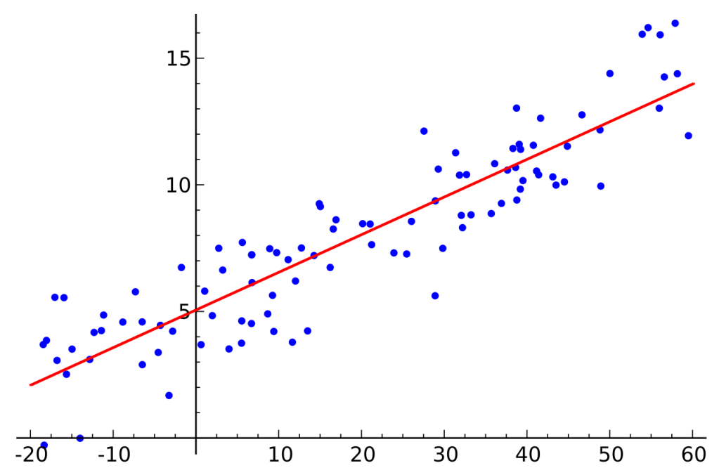
Linear Regression Image credits
Classification
Instead of predicting a range of values, classification predicts categories. Identifying whether an animal is a cat or a dog is a classification problem. Classification algorithms make use of logistic regression. In logistic regression a sigmoid curve is used instead of fitting a linear function to the data.

Sigmoid Curve Image credits
The sigmoid curve is used to give a probabilistic output and based on a suitable threshold the algorithm can predict whether the input falls into a particular category or not.
How to get the best fit?
With both linear and logistic regression, there needs to be a method that optimizes the parameters to give the best fit to the training data. A commonly used method is Gradient Descent.
Imagine you are on top of a valley and your goal is to get to the bottom, so you make a 360 degree turn and take a step in the best direction, and you repeat the process until you have reached the minimum point.
The lowest point of the valley is analogous to the model having the local minimum error i.e. The goal of gradient descent is to minimize the cost function. The cost function is used to calculate the error in the fit used for the training data, and depending on the model we can use a different cost function. Gradient descent essentially iterates on the parameters until convergence i.e. the model has reached the threshold for error.
When the fit is not quite right.
When fitting a function to the data there can be several issues and it is hard to get it right on the first try. The illustration below shows the three possible cases.
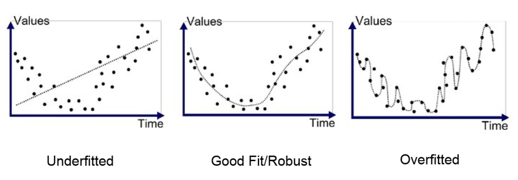
- Underfitted: The order of the polynomial used to fit to the data is too low and it gives inaccurate predictions for the training set.
- Overfitted: The order of the polynomial used to fit to the data is too high. While overfitting ensures that the curve fits well to the training data, it is not robust enough to perform well to changes in the training data.
- Good Fit: The right balance and the order of polynomial is not too high nor too low, which makes the model adaptable to new data as well.
How to Solve the Overfitting issue?
While it may look like an overfit model is a really good fit for the training data, it actually does not perform well when it is introduced to new training data. The following are a few ways to solve this problem.
- Get more training data: With more data points the model is less likely to encounter data that is very different from what it has been trained on. While more data is a simple solution, the problem is getting more quality data can be difficult and the computational time increases.
- Feature selection: Remove certain features from your model. This will reduce the order of the polynomial that fits to the data but you will not account for all the information that you have.
- Regularization: With higher order polynomials, the coefficient of the higher order terms can play a large role in whether the model overfits or not. Regularization is a way to reduce the effect of certain features without completely removing them from the model.
Conclusion
Although I have missed some of the information that I learned from the course and have made multiple mistakes due to flaws in my own understanding of the topics, I do hope that this gives some intuition on how supervised machine learning algorithms actually work.
“Predicting the future isn’t magic, it’s artificial intelligence.”
Dave Waters
